So far this function is only can be used on MS Excel and can not be applied to Google Spreadsheet which is has become my main daily tools for office activity.
As we all know, the VLOOKUP function using syntax:
VLOOKUP(LOOKUP_KEY; VLOOKUP_REFERENCE; INDEX; ISSORTED)
Usually we use VLOOKUP function as seen below:

the cell C5 would be formula to get the price of B4 refer to table F4:G7
using formula
=VLOOKUP(B4;F4:G7;2;0)
But, how if we need to refer the value from an interval value?
For example we need to state a stated remark based on a given value:
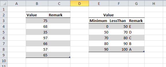
How to do that?
I know you will implement the nested if function such as:
=IF(AND(B3>=E4;B3<F4);G4;IF(AND(B3>=E5;B3<F5);G5;IF(AND(B3>=E6;B3<F6);G6;IF(AND(B3>=E7;B3<F7);G7;G8))))
But I proposed you a different way to get the value using VLOOKUP function below:
=VLOOKUP(B5;{0\"E";50\"D";70\"C";80\"B";90\"A"};2)
I challenge you to try this